Note: This is a a copy of a paper I submitted to a mechanistic interpretability workshop (hence the formality, such as “we” instead of “I”).
The paper can also be found on Arxiv: arXiv:2406.03662
The original project of mechanistic interpretability was a thread of work (Cammarata et al., 2020) trying to reverse engineer InceptionV1 (Szegedy et al., 2014). However, this work had a major limitation that was recognised at the time: polysemantic neurons which respond to unrelated stimuli. It was hypothesised that this was due to superposition, where combinations of neurons are used to represent features (Arora et al., 2018; Elhage et al., 2022). This was a significant barrier to the original Circuits project, since uninterpretable polysemantic neurons were a roadblock for neuron-based circuit analysis.
Since then, significant progress has been made on addressing superposition. In particular, it has been found that applying a variant of dictionary learning (Olshausen & Field, 1997; Elad, 2010) called a sparse autoencoder (SAE) can extract interpretable features from language models (Bricken et al., 2023; Cunningham et al., 2023; Yun et al., 2021).
This creates an opportunity for us to return to the original project of understanding InceptionV1 with new tools. In this paper, we apply sparse autoencoders to InceptionV1 early vision (Olah et al., 2020) and especially curve detectors (Cammarata et al., 2020; Cammarata et al., 2021). We find that at least some previously uninterpretable neurons contribute to representing interpretable features. We also find “missing features” which are invisible when examining InceptionV1 in terms of neurons but are revealed by features. This includes a number of additional curve detector features which were missing from the well-studied neuron family.
Methods
Sparse Autoencoders
Following previous work, we decompose any activation vector into where is the feature activation and is the feature direction. Throughout the paper, we’ll denote these features as <layer>/f/<i> (and neurons as <layer>/n/<i>).
| Layer | Expansion Factor | |
|---|---|---|
| conv2d0 | ||
| conv2d1 | ||
| conv2d2 | ||
| mixed3a | ||
| mixed3b |
Unless otherwise stated, the hyperparameters used for each SAE can be found in Table 1. Our specific SAE setup followed some modifications recommended by Conerly et al. (2024). In particular, we didn’t constrain the decoder norm and instead scaled feature activations by it.11 This seemed to help avoid dead neurons. We also made two additional modifications to work around compute constraints, described in the following subsections.
Over Sampling Large Activations
In InceptionV1, the majority of image positions produce small activations (for example, on backgrounds). To avoid spending lots of compute modelling these small activations, we oversampled large activations by sampling activations from positions in the image proportional to their activation magnitude.
Branch Specific SAEs
InceptionV1 divides these layers into branches with different convolution sizes (Szegedy et al., 2014). For layers mixed3a and mixed3b, we perform dictionary learning only on the 3x3 and 5x5 convolutional branches respectively. This seems relatively principled as with such limited space, features are likely isolated to a branch that has the most advantageous filter size.
Analysis Methods
In analysing features, we primarily rely on dataset examples and feature visualisation (Erhan et al., 2009; Olah et al., 2017). Dataset examples show how a neuron or feature behaves on distribution, while feature visualisation helps isolate what causes a feature to activate. This is supplemented by more specific methods like synthetic dataset examples from Cammarata et al. (2020) for curve detectors.
Dataset Examples
We collect dataset examples where the feature activates over the ILSVRC dataset (Howard et al., 2018), since that is what InceptionV1 was trained on. In using dataset examples, it’s important to not just look at top examples to avoid interpretability illusions (Bolukbasi et al., 2021). Instead, we collect dataset examples randomly sampled to be within ten activation intervals, evenly spaced between 0 and the feature’s maximum observed activation.
Feature Visualisation
Feature visualisation is performed following Olah et al. (2017). We use the Lucent library (Swee Kiat, 2021), with some small modifications to their port of InceptionV1 to ensure compatibility with the original model.22 It was important to us to ensure our model was identical to the one studied by the original Circuits thread. In cross-validating the torch version with the original TensorFlow one, we found that some small differences were introduced to the local response normalisation layer when Lucent ported the model to PyTorch. These significantly modify model behaviour.
Results
This paper is a very early report on applying SAEs to InceptionV1. We present a variety of examples of SAEs producing more interpretable features in various ways. Our sense is that these results are representative of a more general trend, but we don’t aim to defend this in a systematic way at this stage.
Concretely, we claim the following:
- There exist relatively interpretable SAE features which were not visible in terms of neurons.
- There are new curve detector features which fill missing “gaps” among curve detectors found by Cammarata et al. (2020)
- Some polysemantic neurons can be seen to decompose into more monosemantic features.
Each of the following subsections will support one of these claims.
SAEs Learn New, Interpretable Features
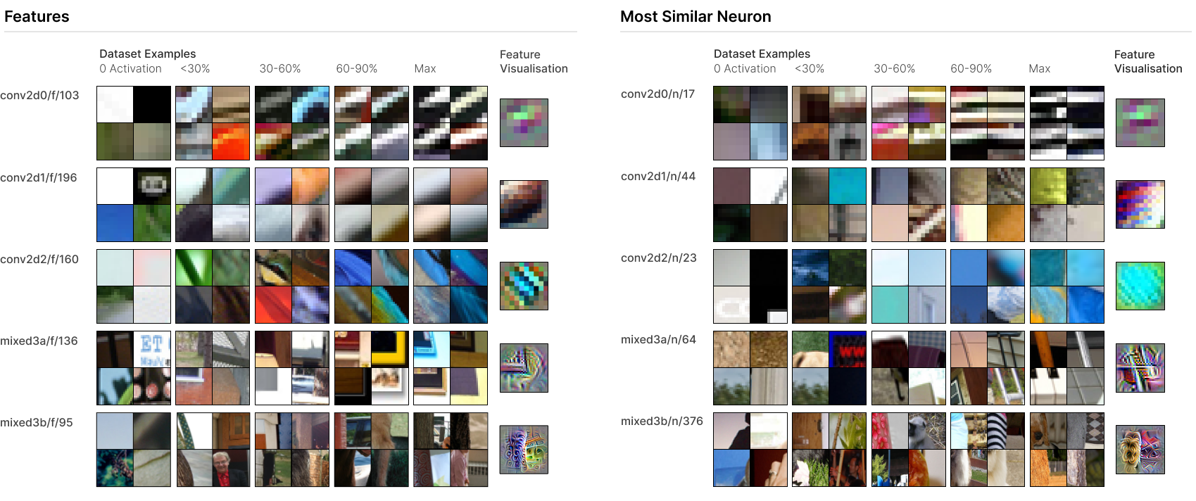
Figure 1 presents five SAE features, one from each “early vision” layer we applied SAEs to. (These are the same five layers studied by Olah et al. (2020).) In each case, the feature is quite interpretable across the activation spectrum (see dataset examples in Figure 1). The neurons most involved in representing the feature are, to varying extents, vaguely related or polysemantic neurons, which are difficult to interpret.
For example, conv2d1/f/196 appears to be a relatively monosemantic brightness gradient detector. However, the most involved neuron conv2d1/n/44 was unable to be categorised by Olah et al. (2020) and appears quite polysemantic. (In fact, our SAE decomposes conv2d1/n/44 into a variety of features responding to brightness gradients of various orientations, colour contrast, and complex Gabor filters.) On the other hand, there are features which have more monosemantic corresponding neurons, but are still more precise and monosemantic. For example, mixed3b/f/95 is a relatively generic boundary detector receiving its largest weight from mixed3b/n/376, which responds to boundaries with a preference for fur on one side. The SAE appears to decompose mixed3b/n/376 into a generic boundary detector and a fur-specific boundary detector in the same orientation.
SAEs Discover Additional Curve Detectors
Curve detectors are likely the best characterised neurons in InceptionV1, studied in detail (Cammarata et al., 2020; Cammarata et al., 2021). They were also found to be concentrated within the 5x5 branch of mixed3b by Voss et al. (2021). This existing literature makes them a natural target for understanding the behaviour of SAEs.
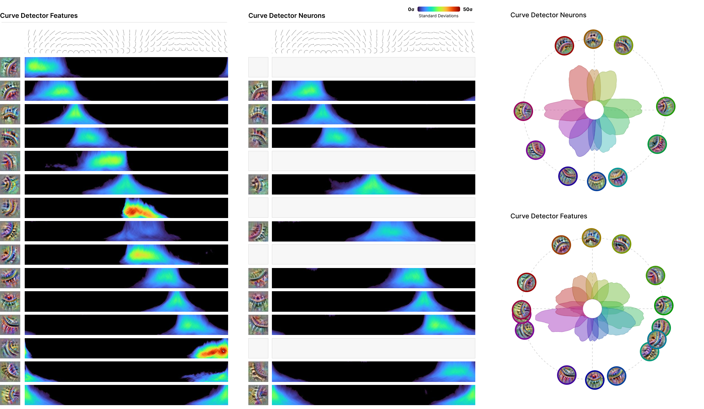
In Figure 2, we use the “synthetic data” approach of Cammarata et al. (2020) to systematically show how our curve detector features respond to curve stimuli of a range of orientations and radii. We find curve detector features which closely match the curve detector neurons known to exist, and others which fill in “gaps” where there wasn’t a curve detector for a particular orientation. Following existing work, we report the stimuli activations in terms of standard deviations to make it clear how unusual the kind of intense reaction they produce is. To see the way the new curve detector features “fill in” gaps, we also create “radial tuning curve” plots from Cammarata et al. (2020), seen in Figure 2. The features fill in several gaps where there is no neuron responding to curves in a given orientation.
SAEs Split Polysemantic Neurons
We’ve already mentioned several examples of polysemantic neurons being split into more monosemantic features. In this section, we’ll further support this pattern with a particularly striking example. Olah et al. (2020) reported the existence of “double curve” detector neurons, which respond to curves in two very different orientations. It’s very natural to suspect these are an example of superposition.
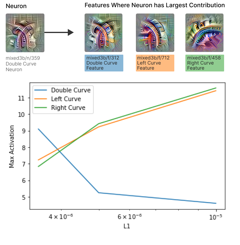
mixed3b/n/359, previously identified by Olah et al (2020) as a double curve detector that was likely polysemantic. Bottom: Max activations of analogous features across SAEs with different L1 coefficients. As L1 increases, the double curve feature becomes smaller, while the left and right curves correspondingly growAs shown in Figure 3, the double curve detector mixed3b/n/359 primarily decomposes into three features: two monosemantic curve detectors and a double curve detector. We suspected the additional double curve detector might be a failure of the SAE. To study this, we trained two additional SAEs with higher L1 coefficients. As L1 the coefficient increases, the maximum activation of the analogous double curve features falls, while the left and right curve features maximum activations correspondingly increases (see bottom of Figure 3).
Conclusion
Recent progress on SAEs appears to open up exciting new mechanistic interpretability directions in the context of language models, such as circuit analysis based on features (Marks et al., 2024). Our results suggest that this promise isn’t limited to language models. At the very least, SAEs seem promising for understanding InceptionV1.
References
Howard, A., Park, E., & Kan, W. (2018). ImageNet Object Localization Challenge.
Arora, S., Li, Y., Liang, Y., et al. (2018). Linear algebraic structure of word senses, with applications to polysemy. Transactions of the Association for Computational Linguistics.
Bolukbasi, T., Pearce, A., Yuan, A., et al. (2021). An interpretability illusion for bert. arXiv preprint arXiv:2104.07143.
Bricken, T., Templeton, A., Batson, J., et al. (2023). Towards Monosemanticity: Decomposing Language Models With Dictionary Learning. Transformer Circuits Thread.
Cammarata, N., Carter, S., Goh, G., et al. (2020). Thread: Circuits. Distill.
Cammarata, N., Goh, G., Carter, S., et al. (2020). Curve Detectors. Distill.
Cammarata, N., Goh, G., Carter, S., et al. (2021). Curve Circuits. Distill.
Szegedy, C., Liu, W., Jia, Y., et al. (2014). Going Deeper with Convolutions. CoRR.
Conerly, T., Templeton, A., Bricken, T., et al. (2024). Update on how we train SAEs.
Elad, M. (2010). Sparse and redundant representations: from theory to applications in signal and image processing.
Elhage, N., Hume, T., Olsson, C., et al. (2022). Toy models of superposition. arXiv preprint arXiv:2209.10652.
Erhan, D., Bengio, Y., Courville, A., & Vincent, P. (2009). Visualizing higher-layer features of a deep network. University of Montreal.
Cunningham, H., Ewart, A., Riggs, L., et al. (2023). Sparse Autoencoders Find Highly Interpretable Features in Language Models.
Marks, S., Rager, C., Michaud, E. J., et al. (2024). Sparse feature circuits: Discovering and editing interpretable causal graphs in language models. arXiv preprint arXiv:2403.19647.
Olah, C., Cammarata, N., Schubert, L., et al. (2020). An Overview of Early Vision in InceptionV1. Distill.
Olah, C., Mordvintsev, A., & Schubert, L. (2017). Feature Visualization. Distill.
Olshausen, B. A., & Field, D. J. (1997). Sparse coding with an overcomplete basis set: A strategy employed by V1?. Vision research.
Swee Kiat, L. (2021). Lucent.
Voss, C., Goh, G., Cammarata, N., et al. (2021). Branch Specialization. Distill.
Yun, Z., Chen, Y., Olshausen, B. A., & LeCun, Y. (2021). Transformer visualization via dictionary learning: contextualized embedding as a linear superposition of transformer factors. arXiv preprint arXiv:2103.15949.
Footnotes
- This seemed to help avoid dead neurons. ↩
- It was important to us to ensure our model was identical to the one studied by the original Circuits thread. In cross-validating the torch version with the original TensorFlow one, we found that some small differences were introduced to the local response normalisation layer when Lucent ported the model to PyTorch. These significantly modify model behaviour. ↩